Overview

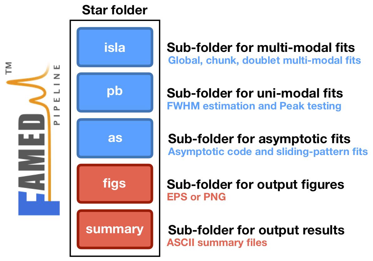
In this section we provide an overview of the outputs produced by the FAMED pipeline from the GLOBAL and CHUNK modules. The figure below shows a sketch of the output folders produced by FAMED. In this section we briefly outline the main and most important outputs produced by the pipeline, namely the figures stored under the folder figs, and the ASCII summary files stored under the folder summary.

The outputs produced by the pipeline are divided into sub-categories. The figure below shows an outline of this scheme. For more details on the file system, check the section File System.

The GLOBAL module

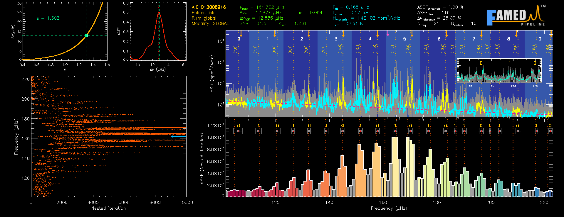
An example of the standard plot output produced by FAMED in the GLOBAL module is shown in Fig. 1. This window shows five different panels.

• On the right side we find on top the plot of the stellar power spectral density (PSD) with a smoothing overlaid in color (cyan and yellow) and the background level shown as well (dashed red line). The position of radial and quadrupole modes is emphasized by the yellow smoothing curve. The global mode identification (either dipole or radial modes and the radial order n) is also overlaid. The orange downward pointing arrows mark the asymptotic predictions of the radial modes, while the purple arrow is \(\nu_\mathrm{max}\). The colored vertical bands depict the individual chunks identified by the module, with corresponding IDs indicated. The inset shows a zoom-in of the central region of the PSD.

• On the right side we find on the bottom the plot of the ASEF, with the angular degree of the individual frequency peaks indicated, as well as the frequency position of each ASEF maximum. The colored bins correspond, with a single color each time, to the extension of the frequency ranges, \(r_\mathrm{a,b}\), around each local maximum. The 1-\(\sigma\) on each individual frequency is indicated.

• On the left side we find on the top-left the \(\Delta\nu\)-\(\epsilon\) diagram, with the yellow curve representing the asymptotic relation by Corsaro et al. (2012)b for red giants, and the teal point and cross marking the \(\epsilon\) prediction obtained for the given star. In the case of stars classified as MS or early SG, this diagram is replaced by the \(T_\mathrm{eff}\)-\(\epsilon\) diagram because of the higher effective temperature of less evolved stars.

• On the left side we find on the top-right the \(\mbox{ACF}^2\) plot for \(\Delta\nu\), obtained as explained in Corsaro et al. (2020) (Sect. 4.2). The red curve shows the \(\mbox{ACF}^2\), while the vertical dashed line indicates the estimate of \(\Delta\nu_\mathrm{ACF}\).

• On the left side we find on the bottom the plot of the sampling evolution of the global multi-modal sampling obtained with DIAMONDS. The arrow marks the position of \(\nu_\mathrm{max}\).

In addition to plotting panels, the output window includes a summary of different computation parameters. These parameters are divided into four groups:

• The first block to the left (yellow) lists the catalog ID (e.g. KIC, TIC, etc.) and star ID of the target of the selected catalog, the output folder of the multi-modal sampling, the output sub-folder of the global multi-modal sampling, and the name of the module being used.

• The second block (green) shows some asymptotic quantities, in particular the value of \(\nu_\mathrm{max}\) used as input, \(\Delta\nu_\mathrm{ACF}\) obtained from the \(\mbox{ACF}^2\) and \(\Delta\nu_\mathrm{fit}\) obtained from the asymptotic fit to the radial modes, \(\epsilon_\mathrm{ech}\) obtained from the sliding-pattern fit, and the curvature term \(\alpha\) also obtained from the asymptotic fit to the radial modes. Finally, this block includes the signal-to-noise ratio of the entire stellar PSD as computed in terms of its smoothing. If the sliding-pattern fit is not used, \(\epsilon\) is obtained from the empirical relations, and \(\epsilon_\mathrm{ech}\) is replaced by \(\epsilon_\mathrm{fit}\) in the summary block.

• The third block (teal) shows other quantities related to the oscillation modes, namely the FWHM used to compute the global multi-modal sampling, \(\Gamma_\mathrm{fit}\), the FWHM of the radial mode estimated from empirical relations at the position of \(\nu_\mathrm{max}\), the upper prior bound on the mode height used for the island peak bagging model, \(H_\mathrm{max,prior}\), and finally the stellar effective temperature \(T_\mathrm{eff}\) that was used as input for the computations.

• The fourth and last block (white) lists a number of values related to the processing of the multi-modal sampling. In particolar we have the threshold (in % of the ASEF global maximum) that is used as the minimum ASEF amplitude variation for locating local maxima by means of the hill-climbing algorithm. In addition we find the total number of bins of the chunk ASEF, the tolerance on \(\Delta\nu\) (in %) for the skimming process (see Corsaro et al. 2020, Sec. 4.5.1), and in conclusion the total number of extracted oscillation frequencies and of identified PSD chunks.

Figure 1. The standard plot output of the GLOBAL module.

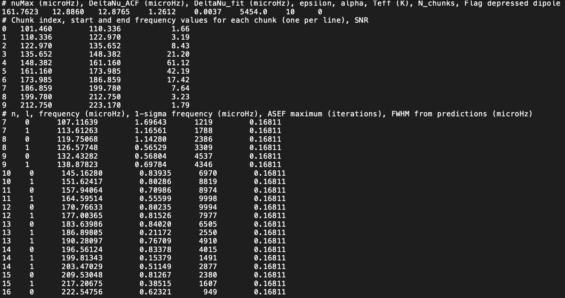
The results computed by the GLOBAL module are stored in an output ASCII file. An example of this output is given in Fig. 2 below. Here the information is divided in three blocks.

• The first block, represented by the first line of values, provides several quantities that are obtained during the computation, such as \(\Delta\nu_\mathrm{ACF}\), \(\Delta\nu_\mathrm{fit}\) from the asymptotic fit (both in \(\mu\mbox{Hz}\)), \(\epsilon\), the curvature term \(\alpha\), the number of chunks identified in the PSD, \(N_\mathrm{chunks}\), and a flag specifying whether the star is a potential depressed dipole star. There also other quantities that have been given as input for the computation, namely \(\nu_\mathrm{max}\) (in \(\mu\mbox{Hz}\)) and \(T_\mathrm{eff}\) (in Kelvin), which are here reported for a summary.

• The second block has a four-column format. Here each line corresponds to a chunk identified by the GLOBAL module. The first column to the left is the chunk ID, the second column is the starting frequency separation (in \(\mu\mbox{Hz}\)), while the third column is the ending frequency separation (coinciding with a starting frequency separation of the next chunk). The last column represents a signal-to-noise ratio evaluated using a smoothed PSD over the level of background.

• The third block has a six-column format. Here each line corresponds to a potential oscillation mode extracted by the GLOBAL module. The first column to the left is the radial order n, the second column is the angular degree (either 0 for radial or 1 for dipole modes), the third column is the oscillation frequency in \(\mu\mbox{Hz}\), the fourth column is the 1-\(\sigma\) uncertainty in \(\mu\mbox{Hz}\), the fifth column is the value of the associated ASEF maximum of the peak as identified by the hill-climbing algorithm, and the last column is a FWHM prediction for the given mode (also expressed in \(\mu\mbox{Hz}\)).

As explained in Corsaro et al. (2020), we remind that the list of global oscillation modes provided by the GLOBAL module is not a definitive list and has to be intended as a preliminary result of low accuracy and precision. For an usable list of frequencies, also for stellar modelling purposes, the user should refer to the output produced by the CHUNK module (see the section below).

Figure 2. The output ASCII file produced by the GLOBAL module.

The CHUNK module

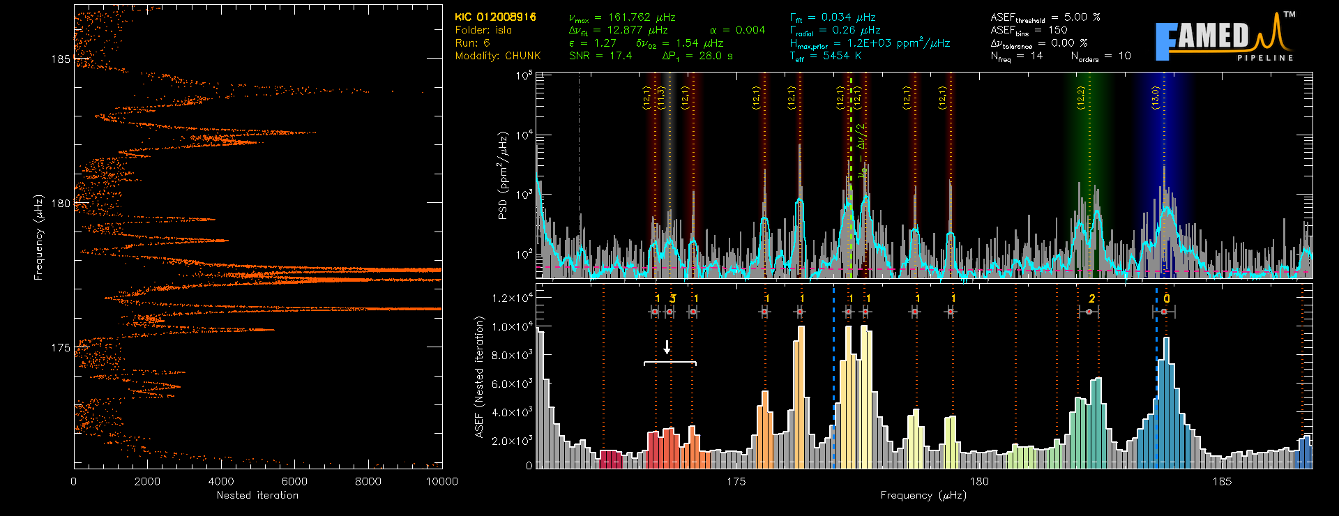
An example of the standard plot output produced by FAMED in the CHUNK module is shown in Fig. 3. This windows shows three different panels, which we describe in the following.

• The panel to the top-right, similarly to the GLOBAL module, represents the stellar PSD in the frequency range of the chunk being analyzed. It shows the stellar PSD in gray, with a smoothing proportional to the linewidth of the chunk radial mode overlaid in cyan color. The vertical shaded bands illustrate the mode identification applied to each frequency peak, with blue showing radial modes, green for quadrupole modes, red for dipole modes, and gray for octupole modes. The mode identification in the form (n,l) as well as the frequency position of the corresponding peak are overlaid. The vertical dot-dashed gray line represents the lower cut to the chunk frequency range used to exclude the region of a potential radial mode belonging to the previous chunk.

• The panel to the bottom-right is the corresponding ASEF, this time obtained from the chunk multi-modal sampling. Here the different colors of the bins, similarly to the GLOBAL module, show the extent of the frequency ranges, \(r_\mathrm{a,b}\), around each local maximum. The 1-\(\sigma\) uncertainty and the angular degree of each oscillation frequency is indicated. In this panel we can also see a white horizontal segment, with a downward pointing arrow, marking the search range of the octupole mode and the corresponding octupole mode asymptotic prediction.

• The panel to the left instead, is the chunk multi-modal sampling evolution, as a function of the nested iterations.

Following the scheme of the GLOBAL module, the CHUNK module lists a number of summary values in the top part of the output window. This information is again divided into four blocks, with blocks in cyan and white showing the same kind of information already described for the GLOBAL module. Here instead

• The first block to the left (yellow) lists the catalog ID (e.g. KIC, TIC, etc.) and star ID of the target of the selected catalog, the output folder of the multi-modal sampling, the output sub-folder of the chunk multi-modal sampling, corresponding to the chunk ID, and the name of the module being used.

• The second block (green) shows some asymptotic quantities, in particular the value of \(\nu_\mathrm{max}\) used as input, \(\Delta\nu_\mathrm{fit}\) and the curvature term \(\alpha\) obtained from the asymptotic fit to the radial modes in the GLOBAL module, the local (chunk) values of \(\epsilon\) and of \(\delta\nu_\mathrm{02}\), the signal-to-noise ratio of the chunk computed in terms of the smoothed PSD, and finally the value of the observed period spacing of dipole mixed modes, \(\Delta P_1\). When either of the parameters \(\epsilon\), \(\delta\nu_\mathrm{02}\), and \(\Delta P_1\) are not available, they are set to 0.

Figure 3. The standard plot output of the CHUNK module.

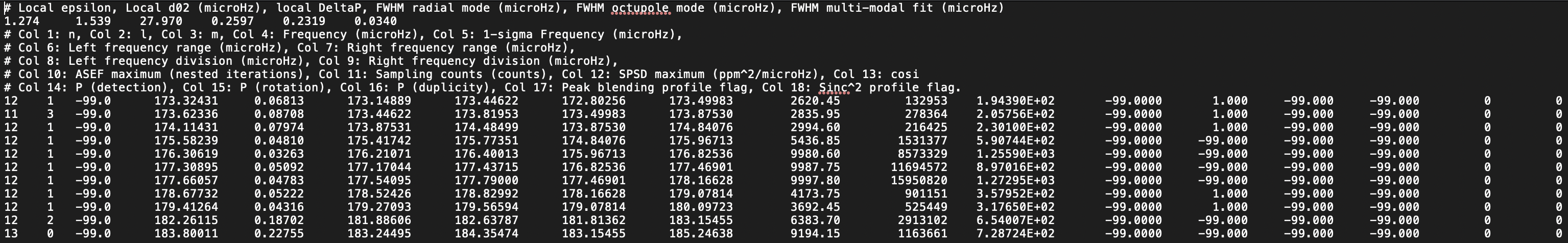
For each chunk analyzed, FAMED produces an ASCII summary file that contains all the useful information computed by the pipeline. An example of this output, corresponding to the chunk shown in Fig. 3, is presented in Fig. 4. This summary file has a two-block structure.

• The first block lists general values stemming from the chunk analysis, in particular the local values for \(\epsilon\), \(\delta\nu_\mathrm{02}\), and \(\Delta P_1\), and the FWHM obtained from the peak fit to the radial mode and possibly to the octupole mode (see Corsaro et al. 2020, Sect. 5.3.1 and 5.5).

• The second block provides a large number of information which corresponds to a single oscillation mode for each line of the file. Most notably, we find find the quantum numbers (n,l,m), the oscillation frequency and its 1-\(\sigma\) uncertainty, the frequency ranges \(r_\mathrm{a,b}\) and divisions \(d_\mathrm{a,b}\), as well as the \(\cos i\) of the star from an individual dipole mode triplet (if detected). The last five columns provide the results from the peak testing phase, thus incorporating probabilities for mode detection, rotation, duplicity, as well as flags specifying whether the mode is a \(\mbox{sinc}^2\) profile and whether it is affected by blending.

The information available for each chunk from the summary file can be exploited for performing a full uni-modal peak bagging analysis in order to obtain oscillation amplitudes and linewidths. We note, however, that individual mode linewidths for all the radial and octupole modes of the star are provided by FAMED already with the CHUNK modality, such that there is no need to rely on further fitting for retrieving these additional oscillation parameters.

Figure 4. The output ASCII file produced by the CHUNK module.